Boston Housing
rpi.analyticsdojo.com
#This uses the same mechansims.
%matplotlib inline
Overview
- Getting the Data
- Reviewing Data
- Modeling
- Model Evaluation
- Using Model
- Storing Model
Getting Data
- Available in the sklearn package as a Bunch object (dictionary).
- From FAQ: “Don’t make a bunch object! They are not part of the scikit-learn API. Bunch objects are just a way to package some numpy arrays. As a scikit-learn user you only ever need numpy arrays to feed your model with data.”
- Available in the UCI data repository.
- Better to convert to Pandas dataframe.
#From sklearn tutorial.
from sklearn.datasets import load_boston
boston = load_boston()
print( "Type of boston dataset:", type(boston))
#A bunch is you remember is a dictionary based dataset.  Dictionaries are addressed by keys.
#Let's look at the keys.
print(boston.keys())
#DESCR sounds like it could be useful. Let's print the description.
print(boston['DESCR'])
# Let's change the data to a Panda's Dataframe
import pandas as pd
boston_df = pd.DataFrame(boston['data'] )
boston_df.head()
#Now add the column names.
boston_df.columns = boston['feature_names']
boston_df.head()
#Add the target as PRICE.
boston_df['PRICE']= boston['target']
boston_df.head()
## Attribute Information (in order): Looks like they are all continuous IV and continuous DV. - CRIM per capita crime rate by town - ZN proportion of residential land zoned for lots over 25,000 sq.ft. - INDUS proportion of non-retail business acres per town - CHAS Charles River dummy variable (= 1 if tract bounds river; 0 otherwise) - NOX nitric oxides concentration (parts per 10 million) - RM average number of rooms per dwelling - AGE proportion of owner-occupied units built prior to 1940 - DIS weighted distances to five Boston employment centres - RAD index of accessibility to radial highways - TAX full-value property-tax rate per 10,000 - PTRATIO pupil-teacher ratio by town - B 1000(Bk - 0.63)^2 where Bk is the proportion of blacks by town - LSTAT % lower status of the population - MEDV Median value of owner-occupied homes in 1000’s Let’s check for missing values.
import numpy as np
#check for missing values
print(np.sum(np.isnan(boston_df)))
What type of data are there?
- First let’s focus on the dependent variable, as the nature of the DV is critical to selection of model.
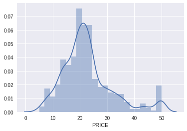
- Median value of owner-occupied homes in $1000’s is the Dependent Variable (continuous variable).
- It is relevant to look at the distribution of the dependent variable, so let’s do that first.
- Here there is a normal distribution for the most part, with some at the top end of the distribution we could explore later.
#Let's us seaborn, because it is pretty. ;)
#See more here. http://seaborn.pydata.org/tutorial/distributions.html
import seaborn as sns
sns.distplot(boston_df['PRICE']);
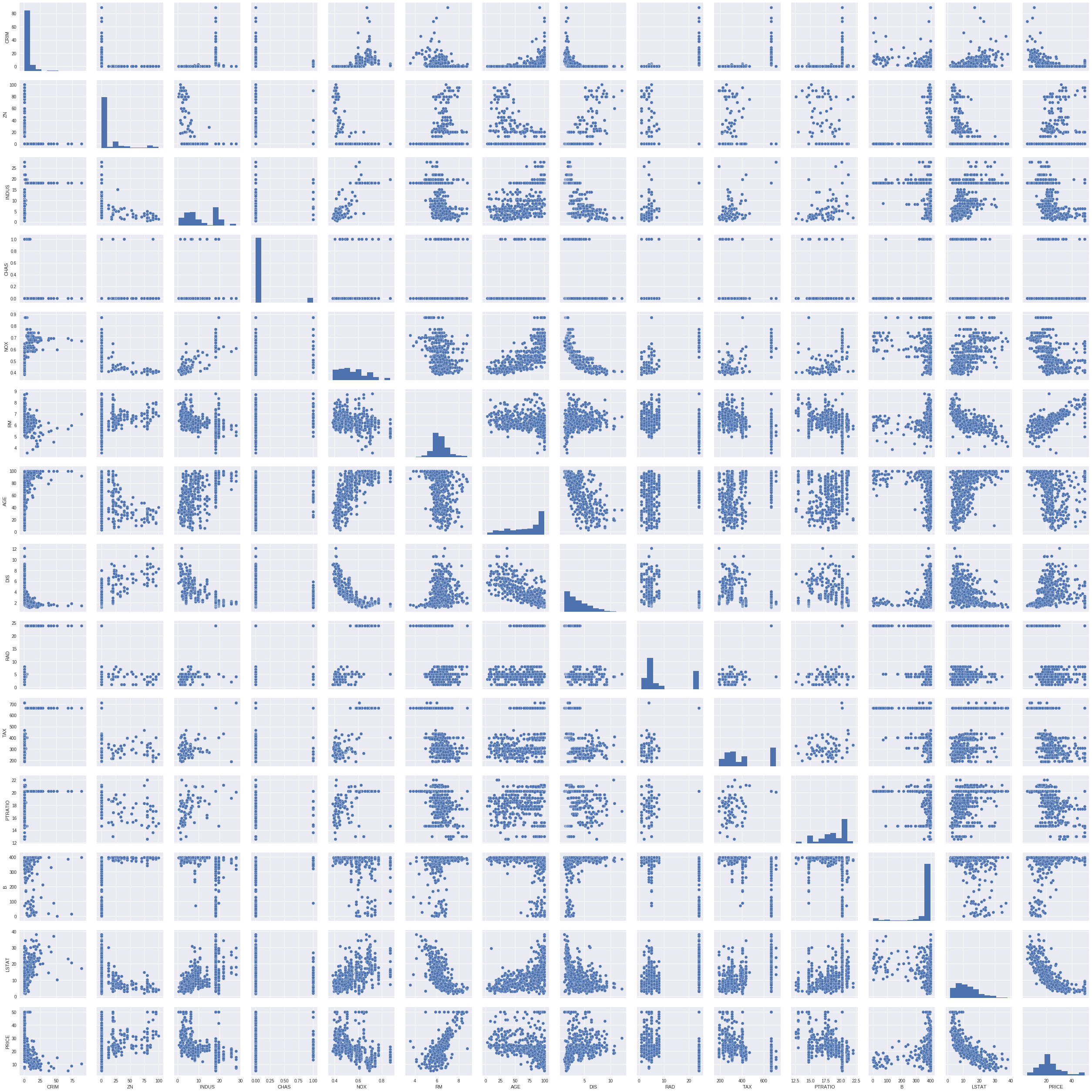
#We can quickly look at other data.
#Look at the bottom row to see thinks likely coorelated with price.
#Look along the diagonal to see histograms of each.
sns.pairplot(boston_df);
Preparing to Model
- It is common to separate
yas the dependent variable andXas the matrix of independent variables. - Here we are using
train_test_splitto split the test and train. - This creates 4 subsets, with IV and DV separted:
X_train, X_test, y_train, y_test
#This will throw and error at import if haven't upgraded.
# from sklearn.cross_validation  import train_test_split
from sklearn.model_selection  import train_test_split
#y is the dependent variable.
y = boston_df['PRICE']
#As we know, iloc is used to slice the array by index number. Here this is the matrix of
#independent variables.
X = boston_df.iloc[:,0:13]

# Split the data into a training set and a test set
X_train, X_test, y_train, y_test = train_test_split(X, y, test_size=0.3, random_state=0)

print(X_train.shape, X_test.shape, y_train.shape, y_test.shape)
Modeling
- First import the package:
from sklearn.linear_model import LinearRegression - Then create the model object.
- Then fit the data.
- This creates a trained model (an object) of class regression.
- The variety of methods and attributes available for regression are shown here.
from sklearn.linear_model import LinearRegression
lm = LinearRegression()
lm.fit( X_train, y_train )
Evaluating the Model Results
- You have fit a model.
- You can now store this model, save the object to disk, or evaluate it with different outcomes.
- Trained regression objects have coefficients (
coef_) and intercepts (intercept_) as attributes. - R-Squared is determined from the
scoremethod of the regression object. - For Regression, we are going to use the coefficient of determination as our way of evaluating the results, also referred to as R-Squared
print('labels\n',X.columns)
print('Coefficients: \n', lm.coef_)
print('Intercept: \n', lm.intercept_)
print('R2 for Train)', lm.score( X_train, y_train ))
print('R2 for Test (cross validation)', lm.score(X_test, y_test))
#Alternately, we can show the results in a dataframe using the zip command.
pd.DataFrame( list(zip(X.columns, lm.coef_)),
            columns=['features', 'estimatedCoeffs'])
Cross Validation and Hyperparameter Tuning
- The basic way of having a train and a test set can result in overfitting if there are parameters within the model that are being optimized. Further described here.
- Because of this, a third validation set can be partitioned, but at times there isn’t enough data.
- So Cross validation can split the data into (
cv) different datasets and check results. - Returning MSE rather than R2.
from sklearn.model_selection import cross_val_score
scores = cross_val_score(lm, X_train, y_train, cv=8)
print("R2:", scores, "\n R2_avg: %0.2f (+/- %0.2f)" % (scores.mean(), scores.std() * 2))
Calculation of Null Model
- We also want to compare a null model (baseline model) with our result.
- To do this, we have to generate an array of equal size to the train and test set.
#Here we need to constructor our Base model
#This syntax multiplies a list by a number, genarating a list of length equal to that number.
#Then we can cast it as a Pandas series.
y_train_base = pd.Series([np.mean(y_train)] * y_train.size)
y_test_base = pd.Series([np.mean(y_train)] * y_test.size)
print(y_train_base.head(), '\n Size:', y_train_base.size)
print(y_test_base.head(), '\n Size:', y_test_base.size)
Scoring of Null Model
- While previously we generated the R2 score from the
fitmethod, passing X and Y, we can also score the r2 using ther2_scoremethod, which is imported from sklearn.metrix. - The
r2_scoremethod accepts that true value and the predicted value.
from sklearn.metrics import r2_score
r2_train_base= r2_score(y_train, y_train_base)
r2_train_reg = r2_score(y_train, lm.predict(X_train))

r2_test_base = r2_score(y_test, y_test_base)
r2_test_reg = r2_score(y_test, lm.predict(X_test))
print(r2_train_base, r2_train_reg,r2_test_base,r2_test_reg  )
Scoring of Null Model
- We got a 0 R-squared for our model. Why 0?
- This is where it is important to understand what R-squared is actually measuring.
- On the left side you see the total sum of squared values (ss_tot_train below).
- On the right you see the sum of squares regression (ss_reg_train).
- For the null model, the ss_tot_train = ss_reg_train, so R-squared = 0.
- By Orzetto (Own work) [CC BY-SA 3.0 (http://creativecommons.org/licenses/by-sa/3.0) or GFDL (http://www.gnu.org/copyleft/fdl.html)], via Wikimedia Commons
#total sum of squares
ss_tot_train=np.sum((y_train-np.mean(y_train))**2)
ss_res_train=np.sum((y_train-lm.predict(X_train))**2)
ss_reg_train=np.sum((lm.predict(X_train)-np.mean(y_train))**2)

r2_train_reg_manual= 1-(ss_res_train/ss_tot_train)

print(r2_train_reg, r2_train_reg_manual, ss_tot_train, ss_res_train, ss_reg_train )
Predict Outcomes
- The regression predict uses the trained coefficients and accepts input.
- Here, by passing the origional from boston_df, we can create a new column for the predicted value.
boston_df['PRICE_REG']=lm.predict(boston_df.iloc[:,0:13])
boston_df[['PRICE', 'PRICE_REG']].head()
Graph Outcomes
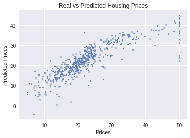
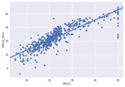
- Common to grapy predicted vs actual.
- Results should show a randomly distributed error function.
- Note that there seem to be much larger errors on right side of grant, suggesting something else might be impacting highest values.
import matplotlib.pyplot as plt
%matplotlib inline
plt.scatter( boston_df['PRICE'], boston_df['PRICE_REG'], s=5 )
plt.xlabel( "Prices")
plt.ylabel( "Predicted Prices")
plt.title( "Real vs Predicted Housing Prices")
#Let's make it look pretty with pickle
import seaborn as sns; sns.set(color_codes=True)
ax = sns.regplot(x="PRICE", y="PRICE_REG", data=boston_df[['PRICE','PRICE_REG']])
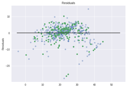
Graph Residuals
- Common to graph predicted - actual (error term).
- Results should show a randomly distributed error function.
- Here we are showing train and test as different
#
plt.scatter( lm.predict(X_train), lm.predict(X_train) - y_train,
           c ='b', s=30, alpha=0.4 )
plt.scatter( lm.predict(X_test), lm.predict(X_test) - y_test,
           c ='g', s=30 )
#The expected error is 0.
plt.hlines( y=0, xmin=-5, xmax=55)
plt.title( "Residuals" )
plt.ylabel( "Residuals" )
Persistent Models
- I could be that you would want to maintain
- The
picklepackage enables storing objects to disk and then retreive them. - For example, for a trained model we might want to store it, and then use it to score additional data.
#save the data
boston_df.to_csv('boston.csv')
import pickle
pickle.dump( lm, open( 'lm_reg_boston.p', 'wb' ) )
#Load the pickled object.
lm_pickled = pickle.load( open( "lm_reg_boston.p", "rb" ) )

lm_pickled.score(X_train, y_train)
Copyright AnalyticsDojo 2016. This work is licensed under the Creative Commons Attribution 4.0 International license agreement.

